Growing cellular automata to visualize DINOv3
What does a vision model see?
DeepDream made me wonder. In 2015, it let an image classifier paint whatever it recognized into any photograph you gave it,1 and the pictures that came out — dogs surfacing in a photograph of clouds — were surreal enough to pull me into computer vision.
A picture like that acts as a hook, turning something unfamiliar into a curiosity worth investigating. Without that kind of window, history shows that people default to fearing what they don’t understand. When ‘big data’ first entered the cultural zeitgeist, many were instinctually afraid of what it meant, and data visualization became a public service. Interactive graphics let anyone look at the data and play with it; no mathematics needed.
Now, this collective fear (if not existential threat) is being projected onto machine learning. I believe interpretability can offer the same kind of public service. Thus far, this hasn’t been the case. Interpretability is a domain obstructed from public view and dominated by shrewd researchers. All that is elevated to the general public is a story about control: a neuron found, a behavior switched off, with nothing to look at or interact with.
To start to fill the gap, I built DinoDreamer, an interactive tool for visualizing DINOv3, Meta’s self-supervised vision model, directly in a browser.
I. Defining the problem: from tokens to pixels
How DINOv3 compresses images, and how a dictionary reads it
DINOv3 is a vision transformer from Meta, trained on 1.7 billion unlabeled images. Yes — not a single image in its training set carries a text label.2
It learns by agreeing with itself. Shown different crops of the same photograph (for example, a crop of the whole car, then a crop of only the wheel), it is trained to ‘summarize’ both the same way.3 To give a wheel and a whole car the same summary, the model has to discover the visual regularities that tie parts to wholes — mapping many varied views onto one compact representation — which is known as compression. Jürgen Schmidhuber has long argued this compression is the core of all learning.4 When given an image, DINOv3 cuts it into patches of 16 by 16 pixels and returns a token for each — a vector of 768 dimensions.
Twelve layers of attention have mixed the rest of the image into each patch token. With DINO frozen, training a single linear layer on top of these tokens gives it the capability to classify the image, segment its objects, or estimate their depth,5 and other models are now built entirely on DINO’s representation space.6 Yet a person cannot read a 768-dimensional vector directly, because a patch’s color, texture, angle, and lighting are entangled across all its coordinates.
The standard tool for decomposing tokens into readable parts is a sparse, overcomplete dictionary: a second, much simpler model that rewrites each token using a small handful of learned entries chosen from a large catalog.7 Think of a kitchen pantry stocked with 16,384 ingredients, where any single dish is made from a short recipe of 32 ingredients at most. In this analogy, each token is a dish, and each dictionary entry is an ingredient.
In the best-known kind of dictionary, the sparse autoencoder, each entry is a single direction in activation space. A single direction can only report one number — how much of that ingredient is present — so any concept that varies continuously gets shattered across separate entries: “Linguine” in one, “Spaghetti” in another, “Rigatoni” in a third.
My dictionary is a block-sparse featurizer, introduced by Thomas Fel and his coauthors this year.8 Instead of a single line, each of its 16,384 entries — a basis group — is a three-dimensional subspace. Ideally, instead of listing “Linguine” as its own ingredient, a basis group can hold “Pasta,” using three internal axes (say, shape, thickness, and dough) to span how pasta varies. When a basis group reads a patch’s token, it projects the 768 numbers onto those three axes to get three coordinates, called the patch’s response: its length indicates how strongly “Pasta” is present, and its direction inside that space indicates whether it is linguine or rigatoni. For each token, the dictionary keeps the 32 active groups with the largest responses, recovering 77% of the variance of held-out tokens — right in line with the 75% Fel and his coauthors report at the same settings, near the threshold where they find downstream “classification and segmentation are essentially unaffected.”9
Plotting a group’s library patches at their three-dimensional responses gives an interactive map of the group, where you can see both its strength and its internal directions at a glance.10
Interact with these basis groups below to see their geometry come to life:



























Where a group fires vs. what makes it fire
Just as a person reads an English dictionary through its usage examples, the usual way to interpret a basis group is to look at the patches it responds to most and name what they share — a guessing game Klindt and his coauthors compare to Connections.11
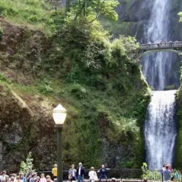
For the two groups above, that game looks straightforward: the strongest images of group 4009 are hibiscus flowers (‘hibiscus’), while group 1304’s two lobes separate ‘dense foliage’ into waterfalls and spruce trees. For other groups, the game breaks down completely. Group 3685 below is a round I could not solve.
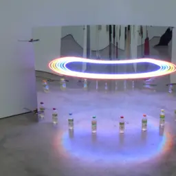

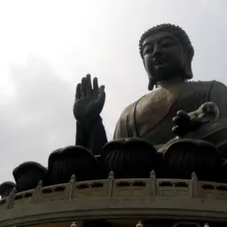
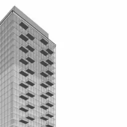
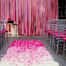


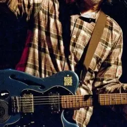
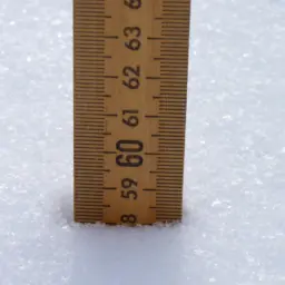





Its strongest patches sit on a violinist, a Minecraft creeper, a water lily, and a ruler stuck in snow; lower on its map are a plate of pasta and a chrome faucet. The language model I used to label all 16,384 groups called it “illustrated faces and figures,” which fits neither the pasta nor the faucet.12
And even when the photographs all show the same object — as they do for ‘hibiscus’ and ‘dense foliage’ — are those hypotheses right? Feature Visualization, the 2017 article by Olah, Mordvintsev, and Schubert that turned DeepDream into a method, posed the problem in four captions under four neurons: “Baseball—or stripes?” “Animal faces—or snouts?” “Clouds—or fluffiness?” “Buildings—or sky?”13 Collecting more dataset photographs cannot settle those questions, because every real photograph bundles the object together with its textures, colors, and lighting. Examples show where a group is firing; they do not show what makes it fire. Rather than collecting more images, the authors proposed synthesizing one by optimization, which “separates the things causing behavior from things that merely correlate with the causes.”
Pixel visualization and the human trap
Synthesizing an image this way is feature visualization; start from noise, and adjust the pixels until the model responds the way you want. I built an interactive painter on it, where you brush a basis group onto part of a canvas to optimize those pixels for the group’s response, with an optional reference image as a prior.
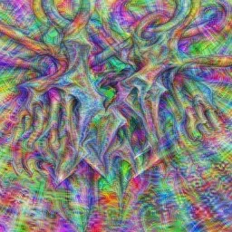
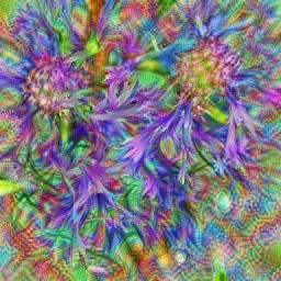
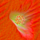
Without the prior (left), I got rainbow static. You can kind of make out flowers and vines in that left panel — but only because you already know it is a flower group and can see the real flowers right beside it. Without knowing what it is supposed to be, you would have no idea.14 That points to a flaw that runs through interpretability: humans seeing what they want to see, rather than seeing a representation for what it is. Left unconstrained, an optimizer that owns every pixel takes the cheapest mathematical shortcut to raise the response, and that shortcut does not have to look like anything to a human.
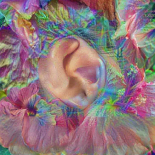
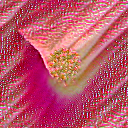
With the prior on (right), you can clearly identify flowers, yet relatable imagery does not mean the visualization is more faithful to the model. In “pollinating season,” below, I painted an ear surrounded by flowers and had to stop the optimization early, because when run to completion the flowers came out too perfect to believe — essentially just my reference image regurgitated back to me.
Feature Visualization arranges methods like these on a spectrum by how heavily they lean on a prior, from adversarial noise at one end to a unit’s strongest photographs at the other — warning that near the photograph end “it may be unclear what came from the model being visualized and what came from the prior.”15 Near that photograph end sits the guide in Nick Cammarata’s 2026 essay Neural Networks Are Already Clean, which steers optimization along the internal routes that the unit’s own strongest photographs take. With my painter, I had walked from one end of the spectrum to the other: from static where I projected what I wanted to see, to a prior where I was looking at the photographs I had brought in.
Of course, the painter was my own code, so I also checked my basis groups with MACO, a modern pixel method that keeps an image’s frequencies close to those of natural photographs.16 Pixel visualization isn’t bad at all. Across most of the groups I tried, MACO found clean structure without collapsing into raw static. For group 3685, maximizing the group’s response drew a field of rounded blobs with areas of illumination within (left below), which I could not yet decipher. When pushed to match DINO’s full tokens on the group’s strongest patches instead (right below), it stitched together a collage of a hand, a small face, and a chair — pieces of my own library images.
Even when a pixel image came out well, the painter failed my wider goal of accessible feature visualization — and it just was no fun to use. Imagine a sketchpad where the ink appears a minute after each stroke. Even on a fast laptop, all it left behind was a single unchanging picture; that latency kills interactability, and if I, the creator of the tool, was growing impatient, there was no hope for anyone else.
II. The method: architectural constraints and the NCA loop
A rule in place of a picture
In a lecture on self-organizing systems,18 Alexander Mordvintsev, one of DeepDream’s three authors, says this about training any differentiable system:
“We always have to remember that loss is always a proxy for a task… It’s always this back and forth process of designing the loss, designing architecture that may implicitly incorporate constraints that you want your system to have…”
Why does optimization need a constraint? Because a loss function is only a proxy for a goal, an unconstrained optimizer will always find the cheapest shortcut to a small number — whether that shortcut is high-frequency static or memorized dataset fragments.19 A constraint limits what the optimizer is allowed to do to satisfy the loss.
With pixel visualization, I had to choose between two extremes in the loss: no image prior (which is interpretable to the vision model, and opaque to a human) or a strong image prior (which is interpretable to a human, only because it forces the image to show what human assumptions demand). I had not yet put the constraint in the architecture. An architectural constraint determines how an image can be constructed, rather than dictating what it must depict. If interpretability is a struggle between the interpretation of the man and that of the machine — wanting the model to represent itself in its own terms (but in a form a person can understand) — architecture offers a middle ground.
Mordvintsev’s lecture was about the neural cellular automaton (NCA), and this is the architecture I employed.20 An NCA is a grid, with one cell per pixel, where each cell sees only itself and its eight neighbors. A small neural network updates each cell based on what it sees — that small neural network is the rule. Every cell runs the exact same rule, just like every cell of a human body carries the same genome, and only the rule is trained.21 Mordvintsev and his coauthors had already trained NCAs to grow textures and to excite single neurons of an older classifier. I added DINOv3 and my dictionary of basis groups.
This architecture became my constraint, and it forces the system to compress. The optimizer that originally owned every pixel now owns none. Every canvas starts from fresh random noise, cells flip a coin at every step so only half update at once, and no cell knows its (x, y) coordinates on the canvas. Deprived of addresses and never meeting the same noise twice, the rule cannot memorize a canvas. Where DINOv3 compresses images into tokens (many-to-one) and the dictionary compresses tokens into three-dimensional basis groups, the NCA rule has to go back from a basis group’s target to a canvas of pixels (one-to-many) through a tiny shared neural network.22 Unable to store a picture by location, gradient descent has to compress whatever the basis group responds to into a local habit — something each cell does with its neighbors, wherever it sits. For this same reason, you can draw on any live canvas on this page; the brush injects fresh noise into the cells it touches, and the rule heals the canvas from that noise.
The back-and-forth: tightening and loosening constraints
In his lecture, Mordvintsev emphasizes that differentiable programming is a continual loop: you design a loss and an architecture, watch what the system does, and go back and forth — altering the architecture, the training regime, and the loss — until the behavior shows you what you are trying to uncover.
To see how that iterative process actually works, walk through it with me on basis group 2632. First, look at the library photographs that activate this group across its four levels of strength:


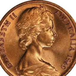

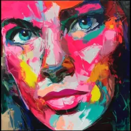
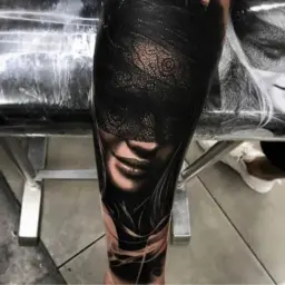
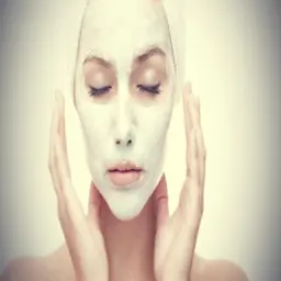

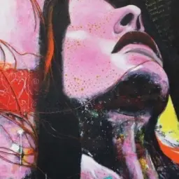
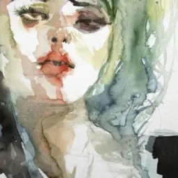
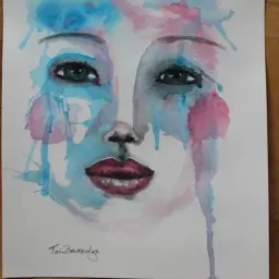



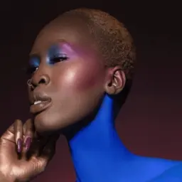
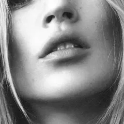
They are all photographs of people, and the active patch consistently lands on the chin or the lips.
I started by keeping the exact same objective I used on pixels — basis-group mean matching, which simply asks the generator to create an image whose patches signal this basis group the same way my target patch does — and only swapped the architecture to a single-grid NCA starting from a noise field.23
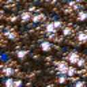
It looks like nothing. Why? Because an NCA’s architectural constraint — where every cell can only talk to its eight immediate neighbors — is so tightly confined to local textures that it struggles to coordinate broader, lower-frequency shapes across the canvas.
What if I loosen that spatial bottleneck and give the rule a way to organize coarser structure? I added a two-grid pyramid: a coarse grid running underneath the fine one, each with its own rule, so cells can coordinate across scales.24
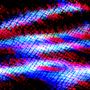
Now it looks like the NCA is actually trying to show something; even on a field of noise, the rule is trying to form the pink, wave-like flow and curvature of lips. Yet because it starts from a noise field — where every cell begins in the exact same situation across the whole canvas — it can only express that curvature as a repeating texture.
What if I give the rule a way to bound a single object, instead of tiling a texture? I changed the start to a noise disc in the center of the canvas (with zeros outside) and propagated the loss through that central area.25 Now that local habit has a boundary to organize around, and on both a single grid and the two-grid pyramid, it finally forms lips:
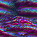
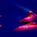
Think about what is happening across these steps in terms of compression and decompression. A basis group is already a compressed representation of what thousands of patches share. When I hold the NCA under a tight constraint — basis-group mean matching, with no guide — I give the rule very limited freedom to visualize. It can only decompress the core meaning of the group: the wave-like flow of lips on a noise field, or an isolated pair of lips on a noise disc.
But constraints do not always have to be tightened. They can be lifted to let the NCA decompress more. I can add an early-training guide (after Nick Cammarata’s 2026 essay, briefly nudging DINOv3’s internal units toward the routes the group’s real photographs take before switching off), or lift the dictionary constraint in the loss itself with token distribution matching (matching DINOv3’s full tokens on the group’s strongest patches instead of only the basis group’s summary).26 Look at what happens on group 2632 when I lift those constraints:
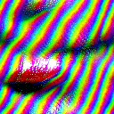
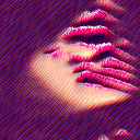
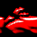
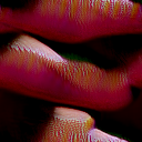

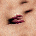
Lifting the constraint lets the NCA decompress much more of the representation: higher visual fidelity, chins, noses, surrounding skin, and whole faces. Yet decompressing further also brings in more correlated baggage, like facial details that happen to sit alongside lips in the library photographs, even though they are not the core concept of the basis group itself. This is the same trade-off I ran into when turning the image prior on and off in pixel visualization. Neither end of the dial is “better” than the other; tightening the constraint isolates the compressed core, loosening it recovers recognizable context, and feature visualization is this iterative back-and-forth.
I wanted anyone reading this to be able to run that loop themselves. Every canvas on this page runs live in your browser on your own device. The site allows you to pick a group, choose the constraints, and train new NCAs right in your tab, with no cloud server behind it (the appendix explains how agent-tuned WebGPU kernels made browser training fast enough to enjoy).
III. The findings: core properties and the limits of dictionaries
Parts and properties: what tight constraints isolate
When I first named basis groups from their library photographs, I fell into the same human habit from Part I; photographs show whole objects and scenes, so I named the groups after nouns.
Once I watched the NCAs grow under tight constraints, I realized why so many of my original noun labels were wrong. A tightly constrained NCA lacks the capacity to decompress an entire scene, so it strips away the correlated objects in the photographs and visualizes only the compressed core — the single part or property that directly satisfies the basis group. Across the sample of basis groups I examined, I renamed more than a third after I watched their NCAs, and nearly all of those new names shifted from a whole object or scene, to an isolated part or property.27 Four specific examples are below. Each opens on the group’s library images, so you can guess the group before clicking the arrow to its NCA.


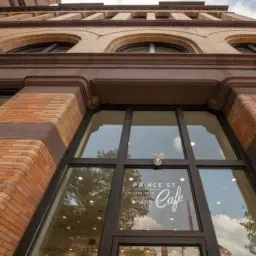



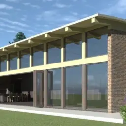
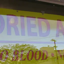

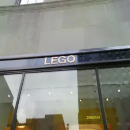



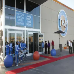
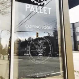
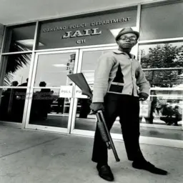
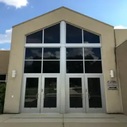
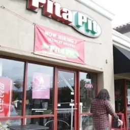

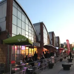
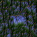
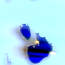

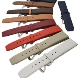
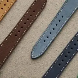
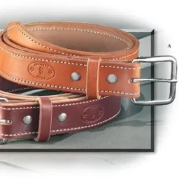


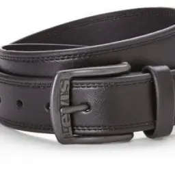



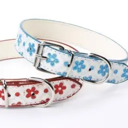

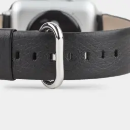





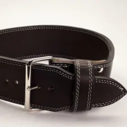
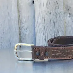
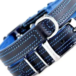
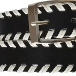
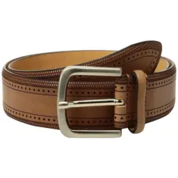
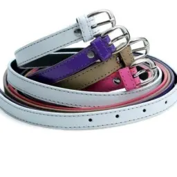

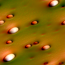
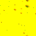
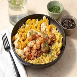

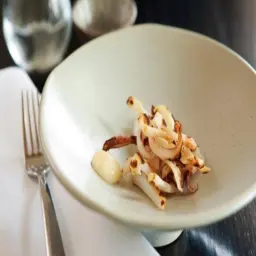
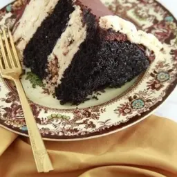
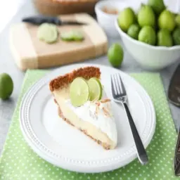
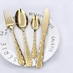

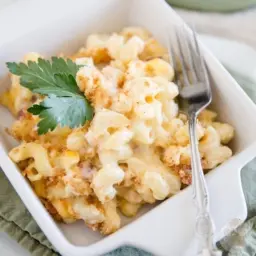
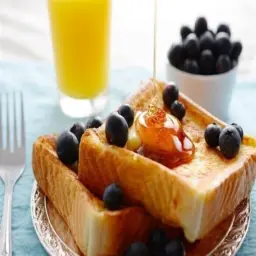
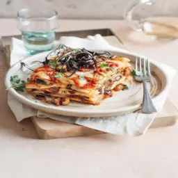

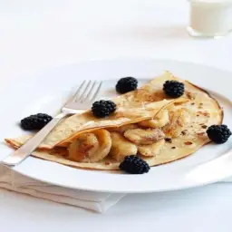
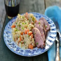
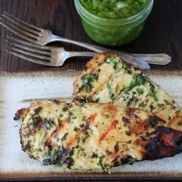




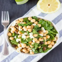
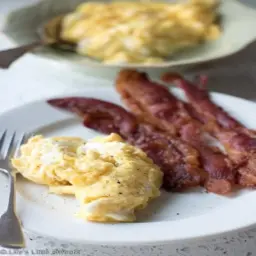
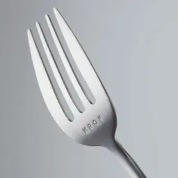



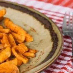
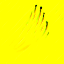
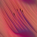
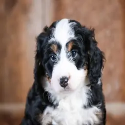

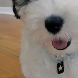

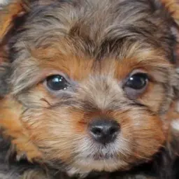
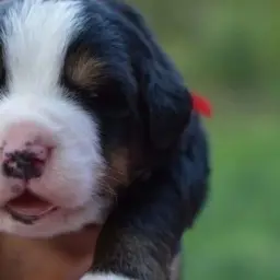
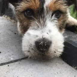
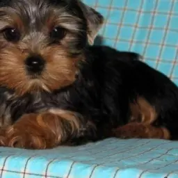
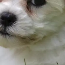



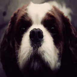


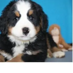




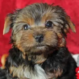
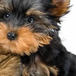

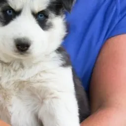
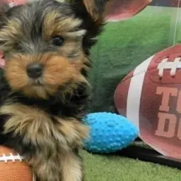
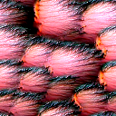
From each set of photographs, I originally named each of these four groups with a specific noun — storefronts, leather belts, forks, puppies. Under the NCA’s bottleneck, the surrounding nouns fall away, and only the core property survives: blue reflections with no storefront behind them, pale holes punched in a brown surface with no belt, thin tines with no fork, pink snouts with whiskers.28 Feature Visualization had asked of one neuron in 2017, “Animal faces—or snouts?” Here, for the puppy group, the NCA answers ‘snouts.’ And because an NCA is a live rule, brushing noise over something like the belt holes tests what the rule prioritizes as it heals; more holes punch straight back through the surface, like whack-a-mole, but never a belt.
That same lens cracked my unsolved Connections round from Part I — group 3685, whose strongest patches sat on a violinist, a Minecraft creeper, a water lily, a ruler stuck in snow, a plate of pasta, and a chrome faucet. What compressed property could those six unrelated photographs share? To find out — and to compare the group’s most compressed core against a slightly loosened constraint — I trained four NCAs for group 3685: two on the left with basis-group mean matching, alone, and two on the right with a guide.
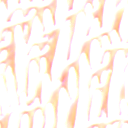
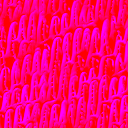
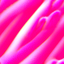
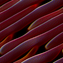
Even on the two unguided canvases to the left, where the rule has only the basis group’s summary to satisfy, you can watch all four develop side by side and brush noise across them — from the flat, pink, shadowy gradients that sweep across a rounded form and build contrast, to bright, lit shapes sitting against the white. When you noise the canvas, it runs that sequence all over again.
The compressed core of group 3685 is shading; the way light falls across a surface and rolls into shadow, whatever that object happens to be. Suddenly the violinist’s cheek, the water lily, the snowbank beside the ruler, the pasta, and the faucet fit together.
The group’s own response over time corroborates this. It responds strongly while the canvas holds a tonal gradient, and stops responding once the canvas bleaches out.29 Even MACO’s earlier pixel image of group 3685 — “rounded blobs with areas of illumination within” — now makes sense in hindsight. MACO drew lit forms too, though it took watching the constrained NCA build and rebuild the gradient from flat pink for me to recognize what I was looking at.
From this, my hypothesis is that many basis groups in the block-sparse featurizer compress a single part or physical property that a great many objects share — a belt, a storefront, or a violinist are simply the correlated context where that property sits in the dataset. Fel and his coauthors found the same thing from the statistical side. In Structuring Sparsity, they rendered twelve 3D models under a moving sun and identified two basis groups in DINOv3 that track illumination across every object (one following scene luminance, one following cast shadow).30 In Into the Rabbit Hull they describe a single DINOv2 token as several properties mixed at once: “a rabbit among animals, brown among colors, fluffy among textures.”31 Of course, my reading is an intuitive inference made by eye, and a local cellular rule naturally favors repeating textures and surface properties.32 What the NCAs gave me was a way to isolate the compressed property without the surrounding nouns getting in the way.
Still a dictionary: when decompression brings the photograph back
Seeing constraints as a dial between compressed core properties and decompressed context also exposes a deeper limit of dictionary-based interpretability: a basis group is a unit the dictionary chose. Whether DINOv3 carves the world into the exact same units is an open question. A different dictionary — or the same block-sparse featurizer trained from another random seed — slices the same 768-dimensional tokens differently, which is why its authors call any featurizer “a hypothesis about the data-generating process of the activations.”33 I chose a block-sparse featurizer so each entry could have a three-dimensional shape, but it is still a dictionary.
Look at how that plays out across the compression dial on group 7705, whose strongest patches all sit on East Asian faces:

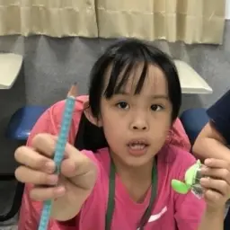
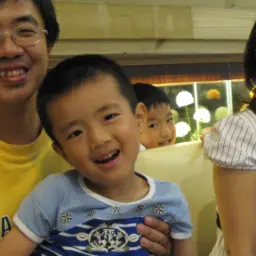


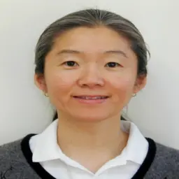
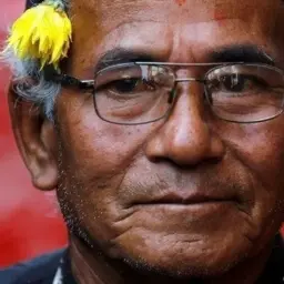



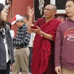
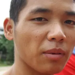




Under a tight constraint — a noise field with basis-group mean matching (left below) — its NCA visualizes only the most compressed core of the group; dark pits in smooth skin, so stripped of context that I could not say what they were. Loosen the constraint one notch — a noise disc with a guide (right below) — and the NCA decompresses just enough surrounding structure to grow a whole head around the pits: black hair, smooth skin, and the exact same dark dots placed where the eyes, the nostrils, and the mouth belong.
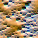
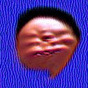
Stepping one notch up the decompression ladder makes the compressed core legible: group 7705 holds the high-contrast dark marks of a face — what is left of a face when you squint. Yet whether those dark marks are one atomic unit to DINOv3, or a mere fragment the dictionary sliced out of something larger, the NCAs cannot tell me.34
So what happens when I lift the dictionary’s constraint out of the loss altogether with token distribution matching — letting the basis group do nothing but pick the reference patches, while the NCA matches the distribution of DINOv3’s full 768-dimensional tokens on those patches and their surroundings?35
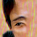
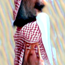
With all 768 dimensions of the tokens in the loss, the NCA decompresses all the way back to high-fidelity objects, along with all their correlated context from the dataset. In the examples above, a detailed face grows for group 7705 (left), and for group 7178 (right) — whose strongest patches sit on men wearing the headdress of the Khaleej — the canvas grows a man in a checked headdress. Both canvases return close to the library photographs themselves, just as MACO’s collage did under the same loss.
That is the two-sided bind of reading a model through a dictionary. Keep the constraint tight on the dictionary’s entry, and you isolate a compressed property — without knowing whether that cut belongs to DINOv3 or to the dictionary. Lift the dictionary constraint to decompress the full tokens, and you bring back the correlated baggage of your own dataset photographs.36
The writer Fabio Morábito describes buying a dictionary from a bookseller who had called it a “stupid dictionary.”37 At home he compared it with the Royal Spanish Academy’s dictionary, the RASD:
I searched for garden in the stupid dictionary: “part of the home, of different shape and size, with plants and flowers, usually surrounded by a fence and for the pleasure of those who inhabit it.” I searched for garden in the RASD and read: “ground where plants are grown for ornamental purposes.” Concise and to the point, and flowers aren’t even mentioned.
My block-sparse dictionary is the Academy’s kind, sparse and compressed by design. Morábito says what such definitions cost is that they “so often imprison us in an endless circle of definitions,” stripping a concept down so far that the flowers aren’t even mentioned. Lifting the constraints on an NCA dials toward the stupid dictionary — putting the flowers back in, along with the fence and the homeowners’ sense of pleasure. Morábito ends the essay by doubting that either end of the dial ever settles a concept alone. Maybe, he writes, “nobody fully understands any word,” with either dictionary.
IV. What this leaves me with
If neither end of the constraint dial settles a concept on its own — if tight compression strips a group down to an isolated fragment and full decompression brings the dataset’s baggage back in — how do you actually read a representation?
In the 1970s, before he wrote Gödel, Escher, Bach, Douglas Hofstadter was a physics graduate student stuck on an equation for electrons in a magnetic field that could be solved only one case at a time, and no individual case showed a pattern. He left the equation alone and changed how he looked at its solutions. A desk calculator worked through the cases, and he plotted every one by hand onto a single sheet of graph paper. Eventually, a butterfly appeared across the sheet, made of smaller butterflies. It led to new theorems, and, 37 years later, experiments found the same butterfly in graphene.38
The butterfly did not live in any single column; it showed up only when all the solutions sat side by side on one sheet. Reading a basis group worked the same way. No single canvas proved what a group was, yet across tighter and looser constraints, I could see which core property stayed while the surrounding context changed.
I believe both differentiable computing and interpretability work best when constraints are treated as this kind of lens; not hunting for one objective or one dictionary label to hand down as a verdict, but varying the bottleneck and comparing the views side by side, the way data visualization does with data.
All 16,384 basis groups are available at dinodreamer.computervision.vision, each with its library images and respective three-dimensional map. Pick a group (or select any patches on a map), choose your start and your loss, train an NCA in your browser on your own device, and draw on what grows. If you like what you grew, you can publish it on the site, or export it as a shader for your own work.
Acknowledgments
I owe the most to two people and one textbook. Alexander Mordvintsev is an author of DeepDream, of the 2017 article on feature visualization, and of the neural cellular automaton. Thomas Fel is an author of five papers behind this project:
- Structuring Sparsity: Block-Sparse Featurizers Capture Visual Concept Manifolds, 2026, which introduced the kind of dictionary I trained.
- Into the Rabbit Hull: From Task-Relevant Concepts in DINO to Minkowski Geometry, 2026, which found concepts that fire away from what drives them.
- Unlocking Feature Visualization for Deeper Networks with MAgnitude Constrained Optimization, 2023, the MACO I compared my NCAs with.
- Feature Accentuation: Revealing “What” Features Respond to in Natural Images, 2024, which starts feature visualization from a natural image.
- Large-scale Neuron Community Discovery Reveals Neuron-Sparse Behaviors in Language Models, 2026, which reads a model through groups of its own neurons.
The project reads Fel’s kind of dictionary with Mordvintsev’s kind of NCA. The textbook is Principles and Practice of Deep Representation Learning, by Sam Buchanan, Druv Pai, Peng Wang, and Yi Ma, open and online. It is where I went to understand how DINO is trained, how representation learning connects to compression, and what a sparse dictionary is.
From Nick Cammarata’s Neural Networks Are Already Clean I took the guide and the test of describing a unit without nouns. Fel and Cammarata both work at Goodfire, and without the research Goodfire publishes, none of mine would be here.
The project also owes something to work that shaped its thinking or that the essay had no place to cite in full:
- Bennett, The Optimal Choice of Hypothesis Is the Weakest, Not the Shortest, 2023.
- Darcet, Oquab, Mairal and Bojanowski, Vision Transformers Need Registers, 2024.
- Didi, The Unification of Representation Learning and Generative Modelling, 2025.
- Fort and Whitaker, Direct Ascent Synthesis: Revealing Hidden Generative Capabilities in Discriminative Models, 2025.
- Gong, Cai, Lin et al., Twins: Learn to Predict Unified Representations with Focal Loss, 2026.
- Gorgun, Schiele and Fischer, VITAL: More Understandable Feature Visualization through Distribution Alignment and Relevant Information Flow, 2025.
- Huh, Cheung, Wang and Isola, The Platonic Representation Hypothesis, 2024.
- Kumar, Clune, Lehman and Stanley, Questioning Representational Optimism in Deep Learning: The Fractured Entangled Representation Hypothesis, 2025.
- Ruthardt, Gaur, Ramanan, Tapaswi and Asano, Steerable Visual Representations, 2026.
- Schmidhuber, Deep Learning: Our Miraculous Year 1990-1991, 2020.
- Schnaus, Dagès, Cremers, Wang and Isola, Shared Geometry As A Rosetta Stone: Cross-Modal Alignment Without Paired Data, 2026.
- Sheppard, Albalak, Lehman and Stanley, Are UFOs Real? Introducing Unified Factored Organizers, 2026.
- Wurgaft, Rager, Kowal et al., Manifold Steering Reveals the Shared Geometry of Neural Network Representation and Behavior, 2026.
- Yang, Xu, Lu, Grossberg, Bai and Shi, Vibe Spaces for Creatively Connecting and Expressing Visual Concepts, 2025.
Finally, a thank you to Yasmine Rayyis who peer reviews my work, writing, and life.
Appendix
A. In the browser
DeepDream spread everywhere in 2015 because the code was public and people could run it on their own photographs. The modern equivalent is a tool that runs directly in a browser tab with nothing to install. To keep DinoDreamer free for everyone, it also had to run without a cloud server behind it, since a hosted GPU costs money on every training run.
Both live replay and full training run locally on your own device. The numerical engine (engine/) is written in Rust on the Burn framework (burn.rs) and compiled to WebAssembly targeting WebGPU.39 It loads DINOv3 ViT-B/16, the block-sparse dictionary, the NCA trainer, and the Adam optimizer onto your local GPU, while the site only serves static files. It trains in Chrome, Edge, and Safari on a laptop or a phone (on an iPhone 16 Pro Max, the site automatically switches from four canvases per update to one).
Once a rule is trained, DINOv3, the dictionary, and Burn are no longer needed to run it, and the NCA turns directly into a self-contained shader. A single cellular step on the 16-channel torus grid applies four fixed filters per channel (the identity, horizontal and vertical Sobel gradients divided by , and the nine-point Laplacian divided by ), passes the resulting numbers through the rule’s two-layer neural network (, bias , ReLU, and ), and adds the update to the cell when a per-cell PCG hash draw (Jarzynski and Olano, 2020) falls below the fire rate. On the page, that entire step runs in one WebGPU compute shader (WGSL), where one GPU thread updates one cell and the first three channels render as RGB color; drawing on a canvas dispatches a small damage shader that blends a soft disc of cells on both grids back toward fresh random noise. Because a trained rule is just float32 weights ( for the two-grid pyramid), the site exports any NCA by writing its weights directly as constant float arrays (const W1 = array<f32, 6144>(...)) inside a standalone .wgsl file. For single-grid rules, it also exports a four-buffer GLSL fragment shader (Buffer A through Buffer D, packing the channels into four vec4 textures that ping-pong between two banks each frame) that runs directly in Shadertoy.
Training in the browser is the expensive half. Each update rolls four canvases forward for to steps, passes two transformed views of each canvas through DINOv3’s twelve attention layers, and backpropagates gradients through DINOv3 and through every step of cellular growth. Out of the box, Burn’s generic tensor operations wrote the perceptions and hidden activations to global GPU memory and read them back several times per step (moving about of global memory traffic per forward step at batch size ), and the fastest NCA took more than two minutes to appear.
To make browser training fast enough to feel interactive, I followed the workflow from Carnegie Mellon’s Agentic GPU Programming for MLSys and gave coding agents an automated verification harness to write and benchmark custom WebGPU kernels in CubeCL and WGSL.40 Every candidate kernel had to pass three automated gates with no person in the loop: a numerical oracle checking forward activations and backward gradients against the PyTorch reference, an alternating ABBA paired clock timing the old and new builds in the same browser session, and a convergence check verifying that the trained NCAs reached the active-patch threshold at least as early as the baseline.
The biggest speedups came from:
- A fused forward step and tape-free chunk backward pass (
cell_step.rs): Keeping the perceptions and hidden activations in of on-chip workgroup shared memory cuts global memory traffic per forward step from to , and recomputing each -step chunk during backpropagation instead of storing an autodiff tape cut total update time by . - An ordered transpose-gather view gradient (
resample.rs): Replacing Burn’s serial scatter-add backward pass on the shifted, scaled, and rotated canvas views with a per-pixel gather in exact source-row addition order cut update time by to . - Rectangular register-tiled projections and on-GPU counter draws (
cell_linear.rs,draws.rs): Matching tile widths to the rule’s narrow - and -channel layers and moving PCG noise and fire-mask generation to the GPU trimmed another to .
Every kept kernel preserves the FP32 training trajectory bit for bit. The fastest rules now appear in about a minute and a half on my laptop.41 The agents wrote the kernels; I decided what had to match, what counted as faster, and when to stop.
B. Architecture and objectives
This section gives the exact specification of the dictionary, the cellular rule, and the four training objectives. Every symbol is defined with its shape and range.
1. Tokens and the block-sparse dictionary
Tokens. DINOv3 ViT-B/16, final-layer patch tokens. A RGB canvas with pixel values in is cut by DINOv3 into patches of pixels. For each patch , let be its final-layer patch token. The reference library holds about images at patches each (about patch tokens).
Dictionary. A Grassmannian block-sparse featurizer with basis groups. Let be the shared token mean, let be the shared scalar scale, and for any token let be the centered and scaled token. For each basis group , let be its orthonormal frame (). The group’s response to token is the three-dimensional projection:
with Euclidean norm . For each token, let with be the set of active groups having the largest response norms , and let be the learned scalar reconstruction gain. The token is reconstructed from its active groups as:
Held-out reconstruction fidelity is .
2. The cellular rule and training loop
Rule. On a single grid with periodic (torus) boundary conditions, let be the state vector of cell . Its first three channels, shifted by and clamped to , define the cell’s visible RGB color; the remaining channels are hidden state. At each step, perception applies four fixed spatial filters (the identity, horizontal and vertical Sobel gradients, and the nine-point Laplacian) to each of the channels, producing a perceived vector . The rule is a two-layer neural network with weights , bias , and output weights ( parameters in total, with no output bias):
Let be an independent Bernoulli draw per cell and step with ; the cell updates asynchronously as:
In the two-grid pyramid, a coarse torus grid of two-pixel cells runs underneath with its own -parameter rule, while the fine rule also receives the upsampled state of the coarse cell beneath it (, adding fine parameters for parameters in total). The displayed image sums the first three channels of the upsampled coarse grid and the fine grid, shifts by , and clamps to .
Training. Rules are trained with Adam over updates, with learning rate on a cosine decay schedule and per-tensor gradient normalization. Each update samples a batch of canvases from a pool of earlier states (replacing one with fresh uniform noise in ), rolls each canvas forward for a random integer step count , and evaluates the loss on two transformed views per canvas (shifted at random by up to pixels, scaled in , and rotated up to ), plus an overflow penalty keeping state channels inside .
3. The four losses and the early-training guide
Let be the set of scored patches on the canvas ( central patches when started from a central noise disc, and when started from a full noise field). Let be the reference set of tokens formed from the basis group’s strongest distinct library images, taking each image’s target patch together with its patch neighborhood ().
Basis-group mean matching. For basis group , let be the group’s response on canvas patch , let be the target response of one strong library patch, and let be the median response norm across library patches where group is active:
Basis-group distribution matching. Let be the group’s response on each reference patch . The loss matches the distribution of canvas responses to the reference set inside via squared maximum mean discrepancy:
where, for finite point sets ,
and averages four Gaussian kernels at bandwidths , with the median pairwise Euclidean distance in .
Token mean matching. Let index four transformer blocks of DINOv3 (zero-based blocks 3, 6, 9, and the final normalized layer 11). For each layer , let and be the patch tokens of the canvas and reference set, standardized per layer by the mean and root-mean-square norm of . The loss matches the mean token across layers:
Token distribution matching. Using the same standardized -dimensional tokens across the four layers , the loss matches the full token distribution with no basis group projection in the objective:
Guide. An auxiliary loss active only during the early updates of training (after Nick Cammarata, Neural Networks Are Already Clean, Goodfire, 2026). It applies a hinge penalty on the internal feed-forward units inside DINOv3 that the group’s strongest library images activate, pulling each unit up toward its activation level on those real images, with its image-space gradient scaled to a fixed multiple of the main loss’s gradient before releasing.
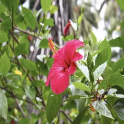
Comparing the losses on one group. The figure below shows four NCAs trained for the hibiscus group, 4009, stepping from basis-group mean matching to basis-group distribution matching and token distribution matching. As the objective constrains more of the token representation, the rule is left with less to invent, and the grown canvas moves from an abstract local motif toward the original photographs.


























Notes
- Mordvintsev, Olah and Tyka, “Inceptionism: Going Deeper into Neural Networks,” Google, 2015. Two years later Olah and Mordvintsev, with Ludwig Schubert, wrote the method up as Feature Visualization, Distill, 2017.
- Siméoni et al., DINOv3, 2025. The images were curated from a pool of about 17 billion collected from public Instagram posts. The model used here, a ViT-B/16, was distilled from the largest of the family, a seven-billion-parameter model: it was trained to reproduce that model’s outputs. The first DINO is Caron et al., Emerging Properties in Self-Supervised Vision Transformers, 2021.
- Two copies of the network, a teacher and a student, see crops of one image. The teacher sees only large crops. The student sees small ones as well, and is trained to summarize each crop the way the teacher summarized a large one. The teacher’s weights are a slowly updated average of the student’s. Since DINOv2, the patch tokens also have a masked-patch prediction task of their own, and DINOv3 adds Gram anchoring to keep patch representations sharp over long training. Yi Ma’s group at Berkeley explain DINO step by step in section 8.2 of their open textbook.
- Jürgen Schmidhuber, “Driven by Compression Progress,” 2009. Yi Ma’s group build their account of representation learning on lossy compression in chapter 4 of their textbook.
- Oquab et al., DINOv2, 2023, and Siméoni et al., 2025, test the frozen tokens this way, with a linear layer for classification, for segmentation and for depth.
- A diffusion model trains faster in DINO’s representation space than in a conventional autoencoder’s: Zheng, Ma, Tong and Xie, Diffusion Transformers with Representation Autoencoders, 2025. Meta’s V-JEPA 2 plans a robot arm’s movements with representations it learned from unlabeled video: Meta, June 2025.
- The idea goes back to sparse coding: Olshausen and Field, 1996. Sparse autoencoders are its most used form in interpretability today: Bricken et al., Towards Monosemanticity, Anthropic, 2023; Cunningham et al., Sparse Autoencoders Find Highly Interpretable Features in Language Models, 2023. Yi Ma’s group derive it as a mixture of overcomplete low-dimensional subspaces in section 2.3 of their textbook.
- Fel et al., Structuring Sparsity: Block-Sparse Featurizers Capture Visual Concept Manifolds, 2026. Using minimum description length, its authors showed that grouping directions into subspaces compresses DINOv3’s activations into fewer bits than single directions do, and found concepts in DINOv3 to be about three-dimensional on average. My dictionary reads DINOv3’s final-layer patch tokens and was trained for three passes over about a million images from MONET and the Describable Textures Dataset. It was learned on the Grassmannian, meaning a group is the space its three axes span, whichever three orthogonal axes are drawn inside it. The weights are on Hugging Face, and the arithmetic is in the appendix.
- In Fel et al., Structuring Sparsity, 2026, Section 3.2 and Figure 6, their Grassmannian featurizer with block dimension b = 3 and sparsity k = 32 reaches a held-out R² of 0.75 (against 0.68 for a single-direction b = 1 featurizer at k = 32), and progressive quantization of DINOv3 tokens shows that linear-probe “classification and segmentation are essentially unaffected down to R² ≈ 0.8.”
- The library is about 650,000 images, or 166 million patches at 256 each, drawn from MONET (Aubin et al., MONET: A Massive, Open, Non-Redundant and Enriched Text-to-Image Dataset, 2026) and the Describable Textures Dataset (Cimpoi et al., Describing Textures in the Wild, 2014).
- Klindt et al., 2026, compare a unit’s examples to the New York Times game Connections, as cited in Tigges et al., Neurons as an Interpretable Basis, Goodfire, 2026.
- Fifteen of the group’s 33 strongest patches lie on the border of their image, and five are the same top-right corner, so the group may partly follow where a patch sits. Fel et al., Into the Rabbit Hull, 2026, find concepts in DINOv2 whose strongest tokens sit away from whatever drives them, and a few that follow position alone.
- Olah, Mordvintsev and Schubert, Feature Visualization, Distill, 2017. The captions are from the figure that sets a neuron’s dataset examples beside an image optimized for it.
- The painter builds its image at five resolutions at once and shifts it a little at every step, both in the spirit of the 2017 work, and the static comes out anyway. Plain gradient ascent on pixels is older: Erhan et al., Visualizing Higher-Layer Features of a Deep Network, 2009.
- Olah, Mordvintsev and Schubert, 2017. One step earlier on the same spectrum, strong regularization “gives more realistic examples at risk of misleading correlations.”
- On November 2, 2026 I ran 198 optimizations on 33 hand-picked groups with plain pixels, a Fourier parameterization and MACO, each with the NCA’s loss, at its size of 128 pixels and with its 1,000 updates. MACO is Fel et al., Unlocking Feature Visualization for Deeper Networks with MAgnitude Constrained Optimization, 2023, which fixes the Fourier magnitude spectrum to that of natural images and optimizes only the phase. In those runs MACO produced something recognizable to me on about 20 of the 33 groups.
- I ran MACO with the settings of its authors’ code: an image 1,280 pixels wide, 1,000 steps, and six random crops at each step. For the second image I used the tokens of the group’s 33 strongest patches, at four of DINO’s layers. A second run of each gave the same kind of image.
- Mordvintsev, Randazzo and Niklasson, Differentiable Self-Organizing Systems, tutorial at ALIFE 2021, July 20, 2021. The quotation is transcribed from the recording, with filler words left out, and the emphasis is mine. Immediately after this passage, he describes altering the loss, the training regime and the architecture in a loop until model behavior moves closer to what you want, and mentions Kenneth Stanley and Joel Lehman’s book Why Greatness Cannot Be Planned, 2015.
- Kumar, Clune, Lehman and Stanley, Questioning Representational Optimism in Deep Learning: The Fractured Entangled Representation Hypothesis, 2025, and Sheppard, Albalak, Lehman and Stanley, Are UFOs Real? Introducing Unified Factored Organizers, 2026, show that optimizing a network toward a fixed objective with conventional gradient descent often yields fractured shortcut representations unless the system is constrained to organize around underlying regularities.
- Mordvintsev, Randazzo, Niklasson and Levin, Growing Neural Cellular Automata, Distill, 2020, and Niklasson, Mordvintsev, Randazzo and Levin, Self-Organising Textures, Distill, 2021. The NCA and its training here follow the second article, whose authors train NCAs to match a texture as the VGG network reads it, and also to excite single neurons of InceptionV1. Treating the generator’s architecture as the prior builds on Mordvintsev, Pezzotti, Schubert and Olah, Differentiable Image Parameterizations, Distill, 2018. Starting every cell as noise follows Pajouheshgar, Xu and Süsstrunk, NoiseNCA, 2024.
- The appendix has the rule in full. A cell holds 16 channels, three of them its visible RGB color and 13 of them hidden channels for signaling. Four fixed 3 by 3 filters on each channel — the identity, the two Sobel gradients and the Laplacian — give the small neural network 64 inputs, and through 96 hidden units it produces 16 outputs that are added to the cell, with probability one half at each step. The rule of a single grid has 7,776 parameters.
- Jürgen Schmidhuber, “Low-Complexity Art,” Leonardo, 1997, formalizes the idea that capturing the essence of an object means finding a short algorithm that generates its regularity rather than storing raw pixel values.
- The appendix gives the loss as a formula alongside the training settings.
- The coarse grid has 64 by 64 cells (each two pixels wide) and the fine grid 128 by 128, for 17,088 parameters in total, adapted from Pajouheshgar, Xu, Abbasi, Mordvintsev, Jakob and Süsstrunk, Neural Cellular Automata: From Cells to Pixels, 2026. On five stubborn groups that had failed to respond on a single one-pixel grid, the two-grid pyramid succeeded in 7 of 10 runs against 2 of 10; across 22 responsive pairs of group and training seed in a second sweep, all 22 responded with two grids.
- The disc is 32 cells across, a quarter of the canvas’s width, and the loss scores the central 4 by 4 patches.
- The appendix defines the guide and all four losses on the site — basis-group mean matching, basis-group distribution matching, token mean matching, and token distribution matching — and compares them on the hibiscus group.
- I picked 33 groups by hand because they looked interesting, went through their NCAs on November 2, 2026, and wrote down what each one showed. For 13 of the 33, the NCA changed the name I had given the group from its images, and for at least nine of those 13 the change went from a scene or an object to a part or a property.
- The test is Nick Cammarata’s. Of a confusing neuron he asks, “if I couldn’t use groups of nouns at all, how would I describe this neuron to someone else?” Neural Networks Are Already Clean, Goodfire, 2026.
- Along a run of the guided noise-disc NCA, the group is active on none of the sixteen central patches at step 25, on 0.41 of them at step 50, on 0.99 at step 100, and on 0.05 by step 500, when a fifth of the canvas is near white (averaged over six runs from different noise). Whether the stopping says something about the group losing its gradient, or about the 32-to-64-step rollout horizon the rule was trained on, I cannot separate from this run alone.
- Fel et al., Structuring Sparsity, 2026, section 5.2. A block is what I call a basis group. Their dictionary is not mine, so I cannot say that group 3685 is either of their two blocks.
- Fel et al., Into the Rabbit Hull, 2026, on DINOv2 with a sparse autoencoder. Among the concepts a depth probe relies on, in the caption of their Figure 6, are “soft lighting gradients and cast shadows.”
- The NCAs also match their three-coordinate target more loosely than pixel methods do: guided NCAs from a noise field end about 0.7 of a median response norm from their target (a squared loss near 0.5), where MACO ends within 0.06 (a squared loss near 0.003) on the runs of November 2, 2026.
- Fel et al., Structuring Sparsity, 2026, crediting Hindupur, Lubana, Fel and Ba, Projecting Assumptions: The Duality Between Sparse Autoencoders and Concept Geometry, 2025. That the cut of a block-sparse featurizer can split a single concept across two basis groups depending on the random seed is shown on synthetic ground-truth data by Jerpelea and Ananthram, A Deeper Analysis of Block-Sparse Featurizers, 2026.
- In the dictionary, group 7705’s nearest neighbor by subspace overlap (the sum of squared cosines of the three principal angles between their frames) is group 9275 (overlap 0.39, against 0.012 for a random pair), whose NCA grows tiny heads from across a room; group 7178’s nearest neighbor is group 13852 (overlap 0.16), whose NCA grows a red-and-white weave where 7178’s grows men in white headdresses. Without training a second dictionary seed, I cannot confirm whether either split belongs to DINOv3 or to the featurizer.
- The distance between the two distributions is the maximum mean discrepancy (MMD) on the tokens of the group’s 33 strongest patches, each taken with the 3 by 3 patches around it, at four of DINO’s twelve layers. The appendix gives all four losses on the site as formulas, and shows the hibiscus group trained across them.
- I also let a single internal unit inside DINOv3 choose the patches in the dictionary’s place: unit 2966 in the feed-forward layer of the tenth block, the one that responds most strongly against its baseline to the patches of group 7178. The NCA grown from that unit’s 33 strongest patches was nothing I could name, and optimizing for a single unit as the whole target did no better.
- Fabio Morábito, “A Stupid Dictionary,” in Mother Tongue, translated by Curtis Bauer, Other Press, 2026, pages 49 and 50. First published in Spanish as El idioma materno, Sexto Piso, Mexico City, 2014.
- Hofstadter, “Energy levels and wave functions of Bloch electrons in rational and irrational magnetic fields,” Physical Review B, 1976; and Gödel, Escher, Bach: An Eternal Golden Braid, 1979. The day he saw the graph is his own telling: “one fine day, to my shock, my eyes suddenly recognized a remarkable type of pattern.” The graphene experiments are Dean et al., Ponomarenko et al. and Hunt et al., all 2013.
- The engine uses the Burn framework and holds DINOv3 ViT-B/16, the dictionary, training and replay. The source is the
enginefolder of the public repository. The NCAs on this page were trained ahead of time with the research code, which is the reference the browser’s trainer is checked against. - Modern GPU Programming for MLSys and Agentic GPU Programming for MLSys, from the MLC community, 2026, both open. The second argues that coding agents can now carry most of the kernel-tuning loop, provided somebody gives them a harness. Their examples are written for NVIDIA hardware with the TIRx compiler. I took the workflow and left the toolchain: a browser has no CUDA, so everything here goes through WebGPU’s shading language.
- Measured in Chrome on an M1 Max on October 22 and 23, 2026, for group 12002 with a single grid from a noise field: 126 seconds before the last round of kernels and 82 after, with an update going from 0.45 seconds to 0.29. Over the six kinds of run on record, the group appeared between 82 and 645 seconds after the click. The oracle’s tolerances were written down beforehand: the gradient at the image, after twelve layers of DINO, has to agree with the reference within 2 percent. One output fusion bought 1.1 percent and made a group that used to appear after 400 updates take 700, so a change that alters one bit of a trained NCA now has to be at least 5 percent faster. The painter’s engine, my first in a browser, went from 2.14 seconds for a step through DINO and back to a tenth of a second in three days, on a slightly lighter workload. The timings are for that laptop and for one desktop with an NVIDIA card. On a phone the site trains one canvas per update.